Notes on Improving Deep Neutral Networks

21 Mar 2020 Machine-Learning

This is the 2nd course of the Deep Learning Specialization on Coursera by Andrew Ng

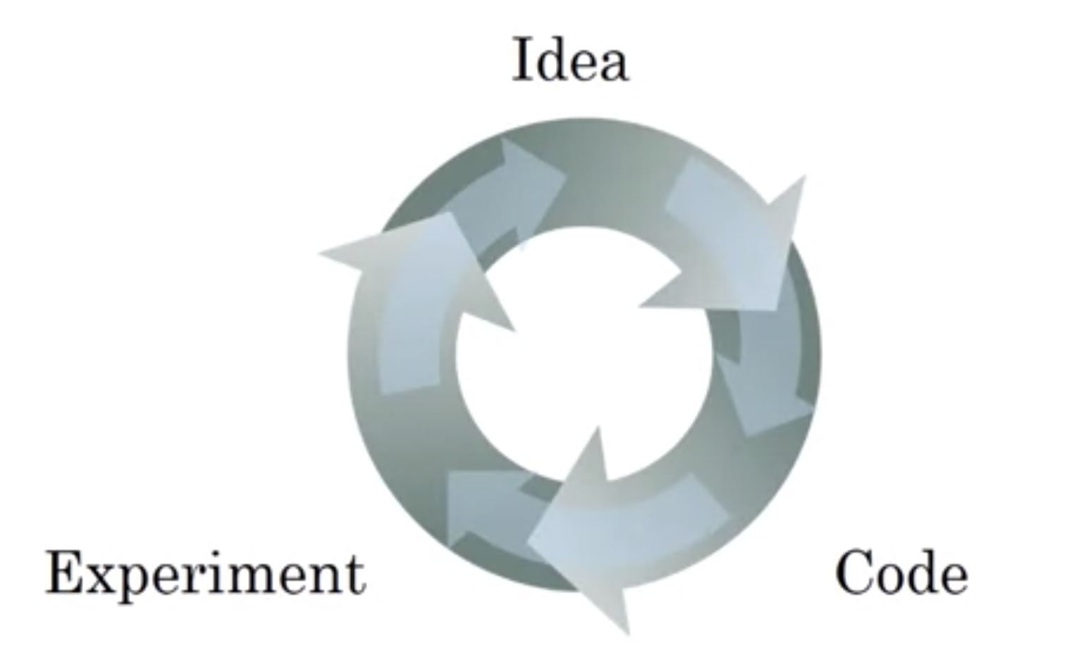
As Andrew Ng has pointed out many times in the course, building machine learning is usually an iterative process with quite some trial and errors. When a ML project starts, it’s better to build and train a simple model quickly, then experiment the model on the dataset to get some sense about the performance. During this process, hopefully you can get more insight of the dataset and understand where the error comes from. This can give you some new ideas to tune the model, or train a new model. This process goes on until you reach the target, usually a sufficiently low prediction error.

ML_iteration

While the first course of this specification introduces the fundamental algorithm and mechanism behind deep learning, the second and third course give more practical instructions when you are dealing with a real ML project. The second course is more about the techniques used to train a better model, i.e., in the trainign phase. The third course, in contrast, talks more about the guidelines and analysing methods used to evaluate the model and further improve the model, i.e., in the evaluation phase. This post will summarize the second course on the training phase (the content of the third course will be given in the next post), and the following points will be addressed:

how to set up ML datasets
why and how to perform regularization for neural network models
how to optimize the parameters in neural network models, i.e., the optimization algorithm
how to tune the hyperparameters
why and how to implement batch normalization

Set up ML datasets

In a typical ML project, you will be given a large amount of data to be used to train your neural network model. After you prepare your data (usually this takes a lot of efforts), the main objective of the training process it to reduce your “cost function” on the dataset by an optimization process of the model parameters (e.g., weights and bias of the neurons).

Hyperparameters However, there are some other parameters that affect the performance of the model and you need to decide before you run the model. These parameters are called hyperparameters. Important hyperparameters for the NN model includes the learning rate, the layer of the the NN, the number of neurons in each layer and the activation function of the neuron, et al. In order to get better hyperparameters, you need to evaluate the model with different hyperparameters on the dataset.

If you evaluate the hyperparameters on the same dataset of training, you have the risk to overfit your data so that it will not give good predictions on the new data, i.e., the model could not generalize well. So it’s better to first separate the dataset into a training set and a holdout/developement/validation set (dev set), and the training set is used to train the model parameters, while the dev set is used to evaluate the hyperparameters.

Furthermore, before you lauch your model into the production line, you need to test your model to get a sense about the generalization error of your final model.

Dataset Division So, the whole dataset is usually divided into three datasets: training set; development set; test set. If the dataset is small (at the scale of 10,000), the training/development/test set can be assigned as 60%/20%/20% of the total dataset. But if the dataset if large (at the scale of 1 million or more), the percentage of data in the dev and test set can be lower, e.g., 1% or so.

Data Shuffle To obtain a good generalization power, it should be ensured that the samples in the dev/test set follow more or less the same distribution. One way to do is first shuffle the whole randomly before you divide the dataset.

Note that the training set does not have to be of the same distribution with the dev/test set. (These points will be further addressed in the next course of this specialization.)

Regularization

Why regularization necessary ?

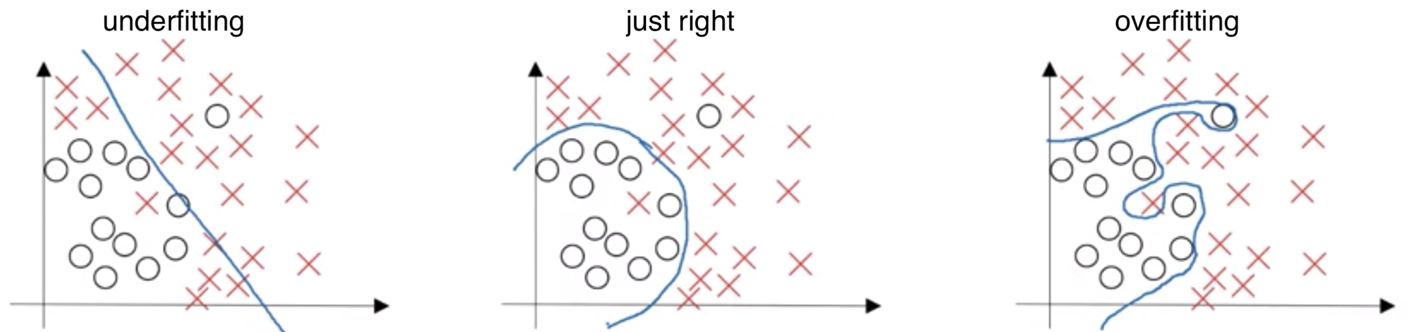
If the training error of you model is about 1%, but the error on the dev set is about 10%, it means that the model does not generalize well, and have a high possibility of overfitting. By overfitting, it means that the model mistakenly captures some subtle unimportant features of the training set, and result in a large variance in the prediction. In the following binary classification problem, the right model overfits the data and gives a very tortuous decision boundary.

overfit_underfit

Regularization by penalty

Mathematical Formulation Adds a Frobenius-norm (not $L_2$ matrix norm) penalization term for the weigh coeffcients in the cost function

$J_{regularized} = \small \underbrace{-\frac{1}{m} \sum\limits_{i = 1}^{m} \large{(}\small y^{(i)}\log\left(a^{[L](i)}\right) + (1-y^{(i)})\log\left(1- a^{[L](i)}\right) \large{)} }_\text{cross-entropy cost} + \underbrace{\frac{1}{m} \frac{\lambda}{2} \sum\limits_l\sum\limits_k\sum\limits_j W_{k,j}^{[l]2} }_\text{L2 regularization cost}$

$\lambda$ is the regularization parameter
In principle, the bias terms $b$ can also be regularized, but in practice, they have much less effect than the weights, so usually omitted.
In the backpropagation step, the weight should be updated by adding an extra $\frac{\lambda}{m}W$ term. This term reduces the weights, so it is also called “weight-decay” regularization.

Why regularization works

(Intuitive way) By regularization, some of the weights are zeroed out, so that the neural network is essentially gets smaller, and less prone to overfitting.
(Mathematical way) By regularization, the weights, in general, become smaller, so that the linear product of the neuron $Z$ is also smaller. For activation functions like $\tanh()$, this means the activation will be more llikely in the linear regime of the function. In general, the whole neural network will be less non-linear, and it will not be able to capture the detailed complicated features.

Dropout

While regularization is a general method that can be used for any machine learning algorithm, dropout is a specific method for neural network to prevent overfitting. It is first proposed in Hinton et al., 2012, and the idea is to randomly shut down some neurons in each iteration. An intuitive explanation why dropout works is that by dropping some of the neurons, a smaller NN is trained so that the problem of overfitting is avoided.

Implementation Firstly, different neurons are dropped for different samples in the dropout method. So this essentially makes some elements of the activation matrix zeros. To implement the dropout, simply apply a mask matrix $M_{\text{dropout}}$ to the neuron activation matrix $A^{[l]}$, where $M_{\text{dropout}}$ is filled with randomly generated ones and zeros so that some of the activations are dropped out. The total number of ones in the matrix is related to the dropout rate you set.

Gradient Checking The idea of gradient checking is to validate the calculation of the gradient in the backpropagation step by the numerical finite difference values. This should be familiar to people who works with differential equations.

Optimization Algorithms

The standard version of batch gradient descent method introduced in last course can be improved in several aspects as follows.

Mini-batch gradient descent

For training large dataset, it is computationally consuming, or even infeasible, to feed all the samples into the net every time to train the parameters (i.e., batch gradient descent). Rather, we can train the model every time using a small number of samples, i.e., mini-batch, and then run through the whole batch in a loop, i.e., epoch. The limiting case is to just use one sample a time to train the model, and this is the stochastic gradient descent.

Implementation Assume the sample matrix and the label matrix with $m$ samples are

$X = [x^{(1)}| x^{(2)} | \cdots | x^{(m)}], \quad Y = [y^{(1)}| y^{(2)} | \cdots | y^{(m)}]$

where $x^{(i)}, y^{(i)}$ represent one sample and its label. We set the mini-batch size as $m_\text{mb}$, and divide the matrix to $n_\text{mb} = \lceil m/m_\text{mb}\rceil$ mini-batches (if not divisible, take the ceiling)

$X = [\underbrace{x^{(1)}|x^{(2)}|\cdots|x^{(m_\text{mb})}}_{\text{mini batch } X^{\{1\}}} | \cdots \cdots | \underbrace{x^{(m - m_\text{mb}+1)} \cdots x^{(m)}}_{\text{mini batch } X^{\{n_\text{mb}\}}}]$

and

$y = [\underbrace{y^{(1)}|y^{(2)}|\cdots|y^{(m_\text{mb})}}_{\text{mini batch } Y^{\{1\}}} | \cdots \cdots | \underbrace{y^{(m - m_\text{mb}+1)} \cdots y^{(m)}}_{\text{mini batch } Y^{\{n_\text{mb}\}}}]$

where the superscript with curly bracket denote the index of mini-batch. Then a typical training process for one epoch would look like

For t in range(1, n_mb+1):
	# Forward propagation using batch t (X^{t})
	# Compute cost for batch t (Y^{t})
	# Backward propagation
	# Update parameters

How it works With mini-batch gradient descent, the hope is that by using a small number of samples, we can still get a good estimation of the gradient with much less efforts. Even though the estimated gradient may not give us the maximum gain in reducing the cost at each step, it makes the computation of each step much faster. So we are trading the number of steps with a fast update at each step, and ideally (and also true in practice), and overall, it reduces the training time. The following picture shows a typical optimization process of batch, mini-batch, and stochastic GD.

descent

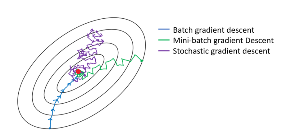
As seen in the figure, the random feature of mini-batch makes the optimization process converge non-monotonically. In another word, the learning curve decreases in a non-monotonical way. This makes the training process difficult to converge to a specific point, but wander around the minimum so that difficult to reach the convergence criteria. Meanwhile, at the beginning of the training, we tend to use large training steps, while at the end of the traing as the learning approaches the minimum, we tend to use small steps.

To do this, we can add learning rate decay, i.e., slowly reduce the learning rate during training. For example, the learning rate $\alpha$ can be updated by

$\alpha = 0.95^\text{number of epoch} \alpha_0,$

where $\alpha_0$ is the initial value of learning rate.

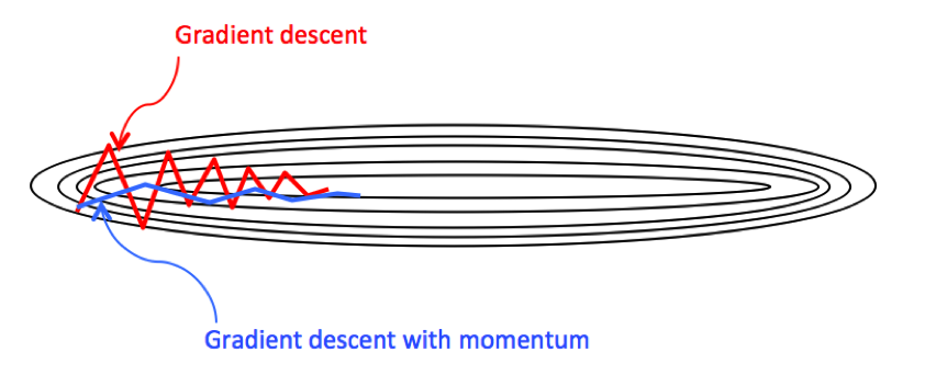
Gradient descent with momentum

Another way to improve GD is to average the newly updated parameters with the old ones. The intuition here is that by averaging the off-the-target components of the gradient vector will be reduced, so that the convergence will be accelerated. Formally, it can be implemented using the exponentially weighted average.

GD_momentum

Exponentially weighted average Assume $\theta_t$ is the gradient vector calculated by backward propagation at time step $t$, and $v_t$ is the exponentially weighted average of $\theta_t$, $v_t = \beta \; v_{t-1} + (1 - \beta) \; \theta_t$

$\beta$ is a hyperparameter controlling the latency of the average. The larger $\beta$ is, the higher are the weights on the past. Typically $\beta = 0.9$ .
the estimated duration of the average is about $\frac{1}{1 - \beta}$
if $\theta_0$ is set to $0$, the first few terms of $v_t$ will be underestimated, to compensate this effect, we add a bias correction step as $v_t = v_t/(1-\beta^t)$. Obviously, with the increase of $t$, the correction will be exponentially smaller, and plays no role.

Following the idea, the update of parameters in GD with momentum and bias correction is written as

$\begin{aligned} V_{dW} & = \beta \; V_{dW} + (1-\beta) \; dW \\ V_{db} & = \beta \; V_{db} + (1-\beta) \; db \\ V_{dW} & = \frac{V_{dW}}{1 - \beta^t} \\ V_{db} & = \frac{V_{db}}{1 - \beta^t} \\ W & = W - \alpha \; V_{dW} \\ b & = b - \alpha \; V_{db} \end{aligned}$

More mathematical details about GD with momentum can refer to Matrix Methods course by Prof.Gilbert Strang. Although there is some gap between the simple example discussed there and the real scenario in NN, it is still helpful in getting the general picture of this method. I’ll see if I can get some research papers in the context of NN on this point.

RMSprop

The RMSprop method looks similar to the exponentially weighted average with the linear term replaced by squared one,

$\begin{aligned} S_{dW} & = \beta \; S_{dW} + (1-\beta) \; dW^2 \\ S_{db} & = \beta \; S_{db} + (1-\beta) \; db^2 \\ S_{dW} & = \frac{S_{dW}}{1 - \beta^t} \\ S_{db} & = \frac{S_{db}}{1 - \beta^t} \\ W & = W - \alpha \; \frac{dW}{\sqrt{S_{dW}} + \epsilon} \\ b & = b - \alpha \; \frac{db}{\sqrt{S_{db}} + \epsilon} \end{aligned}$

Adam

Adam is actually the combination of GD with momentum and RMSprop. Formally, it is written as

$\begin{aligned} V_{dW} & = \beta_1 \; V_{dW} + (1-\beta_1) \; dW, \quad V_{db} = \beta_1 \; V_{db} + (1-\beta_1) \; db \\ V_{dW} & = \frac{V_{dW}}{1 - \beta_1^t}, \quad V_{db} = \frac{V_{db}}{1 - \beta_1^t} \\ S_{dW} & = \beta_2 \; S_{dW} + (1-\beta_2) \; dW^2, \quad S_{db} = \beta_2 \; S_{db} + (1-\beta_2) \; db^2 \\ S_{dW} & = \frac{S_{dW}}{1 - \beta_2^t}, \quad S_{db} = \frac{S_{db}}{1 - \beta_2^t} \\ W & = W - \alpha \; \frac{V_{dW}}{\sqrt{S_{dW}} + \epsilon}, \quad b = b - \alpha \; \frac{V_{db}}{\sqrt{S_{db}} + \epsilon} \end{aligned}$

Hyperparameter tuning

In the NN model, there are quite a lot hyperparameters, for example,

the learning rate $\alpha$
the number of layers
the number of hidden units in each layer
the mini-batch size
the tuning parameters in the GD momentum or Adam, $\beta, \beta_1, \beta_2$

Grid search vs Random search

To find the best hyperparameters, it is usually a practise to perform a grid search in the parameter space in the classical machine learning approach. However, in the deep learning approach, since there are a lot of hyperparameters, and often these parameters are of different significance to the model (think of the learning rate $\alpha$ compared to the momentum parameter $\beta$). If a grid search is used, the change of the less significant hyparameters will give very similar results and it is a waste of computational resources. So, it is generally better to do a random search in the NN model.

It should be noted that “random” search does not have to uniformly random. For some of the hyperparameters, whose range is at the same order of magnitude, e.g., the number of hidden units between 50 to 100, it is reasonable to use a uniformly random search.

For some hyperparameters which range across several order of magnitudes, it is better to perform a random search on the log scale. For example, the learning rate $\alpha$ is typically between $10^{-4}$ and $1$,

r = -4*np.random.rand()  # generate a random number between (0, 4)
alpha = 10**(-r)

Batch normalization

Think of the feature scaling/normalization of the training dataset, it makes the training process easier shown below

normalization

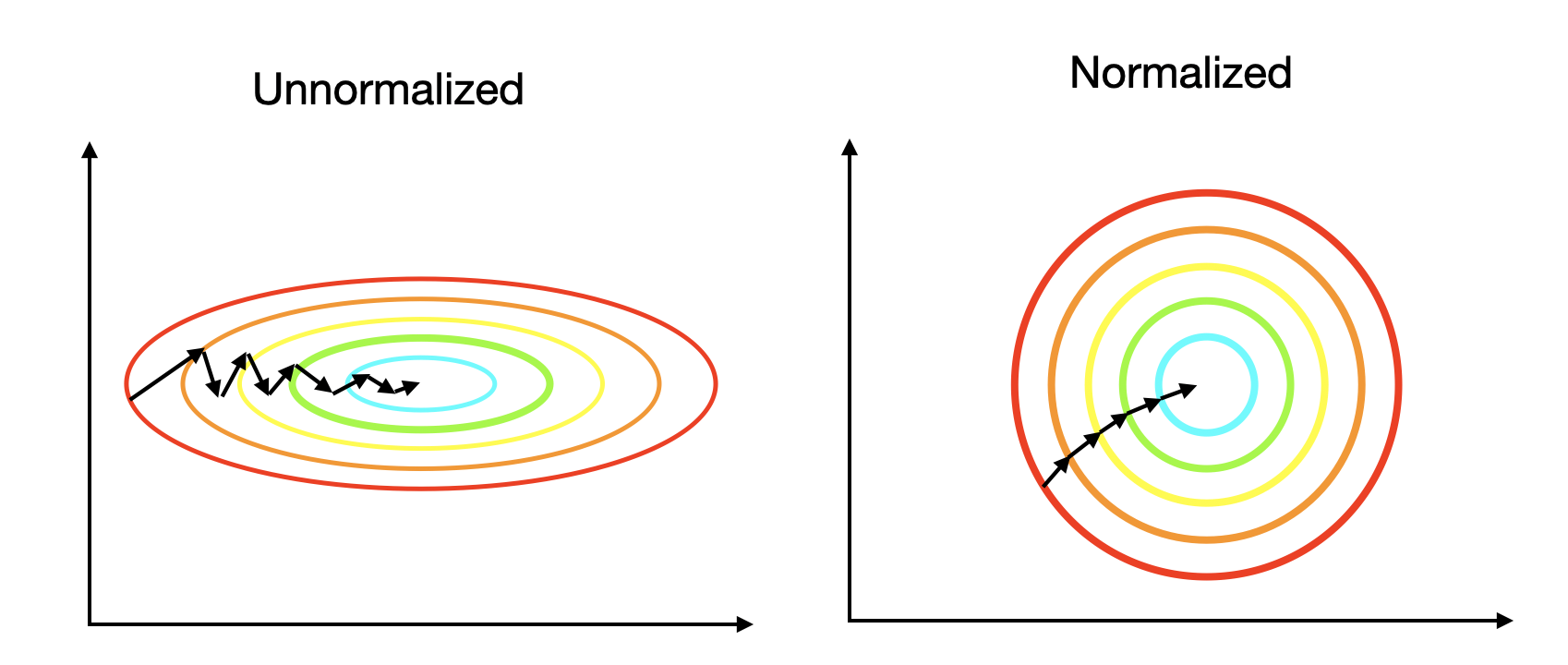
Inspired by this idea, batch normalization is to normalize the activation $a^{[l]}$ before it is fed into the next layer.

Batch normalization makes your hyperparameter search problem much easier, makes your neural network much more robust. The choice of hyperparameters is a much bigger range of hyperparameters that work well, and will also enable you to much more easily train even very deep networks

Implementation Technically, in batch normalization, it is the output $z^{[l]}$ to be normalized $z^{[l]}_{\text{norm}} = \frac{z^{[l]} - \mu}{\sigma + \epsilon}$ where $\mu = \frac{1}{m} \sum\limits_i z^{[l](i)}, \quad \sigma^2 = \frac{1}{m} \sum\limits_i (z^{[l](i)} - \mu)^2$ and $\epsilon$ is a small parameter to avoid the divided-by-zero error.

In practice, rather than a normal distribution, it is common to rescale the distribution with learnable parameters ($\gamma, \beta$ below), e.g., $\tilde{z}^{[l]} = \gamma \; z^{[l]}_\text{norm} + \beta.$ Take the sigmoid activation as an example, usually you don’t want $z^{[l]}$ always locate in a small region around 0, where the sigmoid activation si similar to a linear function.

A bit more about BatchNorm From a theoretical point of view, batch normalization actually has two benefits for the model. Firstly, it reduces the effect of “covariate shift” for the deeper layers by separating the interaction between the layers. Secondly, it has a slightly regularization effect by adding noice to each layer’s values $z^{[l]}$ in the mini-batch because it normalizes each mini-batch differently.

At test time, rather than a mini-batch, maybe you only get one sample a time to feed in the model, thus you don’t have enough samples to compute the mean $\mu$ and variance $\sigma$. So, instead of computing $\mu$ and $\sigma$ in time, they are recorded in the training process, and updated, for example, the exponentially averaing method. In this way, after the training, you will have fixed $\mu$ and $\sigma$ for each layer.

In Keras, there is a BatchNormalization wrapper layer performing batch normalization.

References

https://www.coursera.org/learn/deep-neural-network/home/welcome
https://www.youtube.com/watch?v=wrEcHhoJxjM
https://keras.io/layers/normalization/

集虚斋